The Cosmic Microwave Background (CMB) has provided us with information on the origin of the Universe since it is the oldest electromagnetic radiation we can measure. Similarly, there exists a Gravitational Wave Background (GWB) which is a superposition of gravitational waves generated by different astrophysical and cosmological sources, and can go even further back in time than the CMB, due to the weak coupling of gravitational waves (GWs) and matter. Examples of astrophysical sources include distant compact binary coalescences (CBCs) that cannot be resolved individually and core collapse supernovae. We now have a prediction for the range of strengths of the background originating from distant CBCs, but the background from core-collapse supernovae currently has unknown amplitude, though it is sure to exist. In addition, there are some more speculative sources such as cosmic strings, inflation and first order phase transitions, which are a few examples of cosmological sources. Detecting any of these GW background sources would be a major breakthrough and would provide fundamental insights into astrophysical and/or cosmological processes.
We analyzed data from the first three observing runs (O1, O2 and O3) of Advanced LIGO and Advanced Virgo. We were unable to claim a detection, though we placed more stringent upper limits on the strength of the GWB than had been published before, due to the inclusion of the latest O3 data (see Figure 1). We improved the sensitivity of our search by applying a procedure to remove excess noise. During this procedure we ensured that – to the best of our knowledge – there was no correlated signal coming from environmental noise, such as instrumental, geological or human-related sources. Furthermore, we mitigated the effect of loud glitches by a technique called gating, used for the first time in the search for a GWB, but a standard technique in CBC searches. It consists of zeroing out each glitch in the time domain. This is also the first time that we have included data from the Virgo interferometer in addition to the two LIGO instruments when searching for the GWB. Data from these interferometers was cross-correlated and then used to determine the 95% credible level upper limit on the GWB amplitude through Bayesian inference. Cross-correlating the data allowed us to remove the remaining environmental noise from our analysis, assuming it is un-correlated between interferometers. Co-aligned and co-located detectors are the most sensitive to a GWB, but also to local noise sources. Therefore, the sensitivity to the GWB is dominated by the pair of LIGO detectors, which are the closest to being co-aligned and co-located, though they still provide significantly less than the maximum sensitivity. The contribution of the Virgo detector to the sensitivity is only a few percent, due to its distance and orientation compared to those of the LIGO detectors. Thanks to the relentless efforts of all scientists improving the interferometers, our current upper limit is about a factor of 5 better compared to previous results. While part of this improvement is simply due to analyzing a larger amount of data, most of the increase was due to the increase in sensitivity. If the interferometers had operated at the same sensitivity as in O2, the additional data would only have led to an improvement in the upper limit of less than a factor of 2.
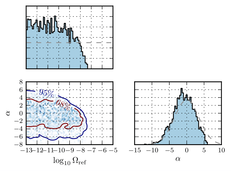
Figure 1: Plot showing the probability distributions for the amplitude of the gravitational wave background Ωref and the spectral index α in Ωref(f/25 Hz)α, our assumption about the GWB dependence on frequency f (which includes the frequency dependence of a number of possible sources). These distributions show that the data prefers lower values of Ωref. The grey dashed lines represent our “a priori” assumptions about these parameters. The 68% and 95% curves show the regions enclosing those percentages of the total probability.
We have also searched for globally correlated magnetic noise, known as Schumann resonances, by looking at magnetic field measurements using dedicated sensors placed near the three interferometers. Identifying Schumann resonances is necessary because they can appear as an effective background and thus “pollute” our signal. The magnetic fields couple to critical parts of the interferometer, e.g., the magnets on the end mirrors, used to control the mirrors and therefore the interferometer. If this coupling is strong enough, it can fake an observable signal where the mirror displacement is not due to a passing GW but due to magnetic fields. Consequently, the Schumann resonances may cause high correlations that could lead us to wrongly claim a GWB detection. To construct a prediction of possible magnetic contamination (see Figure 2) we need two key ingredients. The first is accurate on-site magnetic field measurements with dedicated sensors. The second is a measurement of how these magnetic fields couple to our interferometers and therefore have the possibility to enter as a “fake GW signal”. To determine this coupling we use a coil to create strong magnetic fields near the interferometer and observe their effect on the inferred fake GW signal, while also measuring the magnetic fields accurately. We test for magnetic contamination in two ways. First, we look for contamination in individual frequency bins. Second, we look for the possibility that the sum of magnetic contamination in different frequency bins accumulates to give a result that is above our sensitivity. Our conclusion is that our measured estimates of correlated magnetic noise are well below the sensitivity we achieved in O3, both in individual frequencies and accounting for a sum over multiple frequencies (see Figure 2). Additionally, we implemented a framework, based on Bayesian inference, to simultaneously fit for a GWB and Schumann resonances in our data. Consistent with our other methods, we find neither a signal from the GWB nor one from Schumann resonances. Nevertheless, this newly developed framework is expected to prove extremely useful in future searches as our sensitivity increases even further.
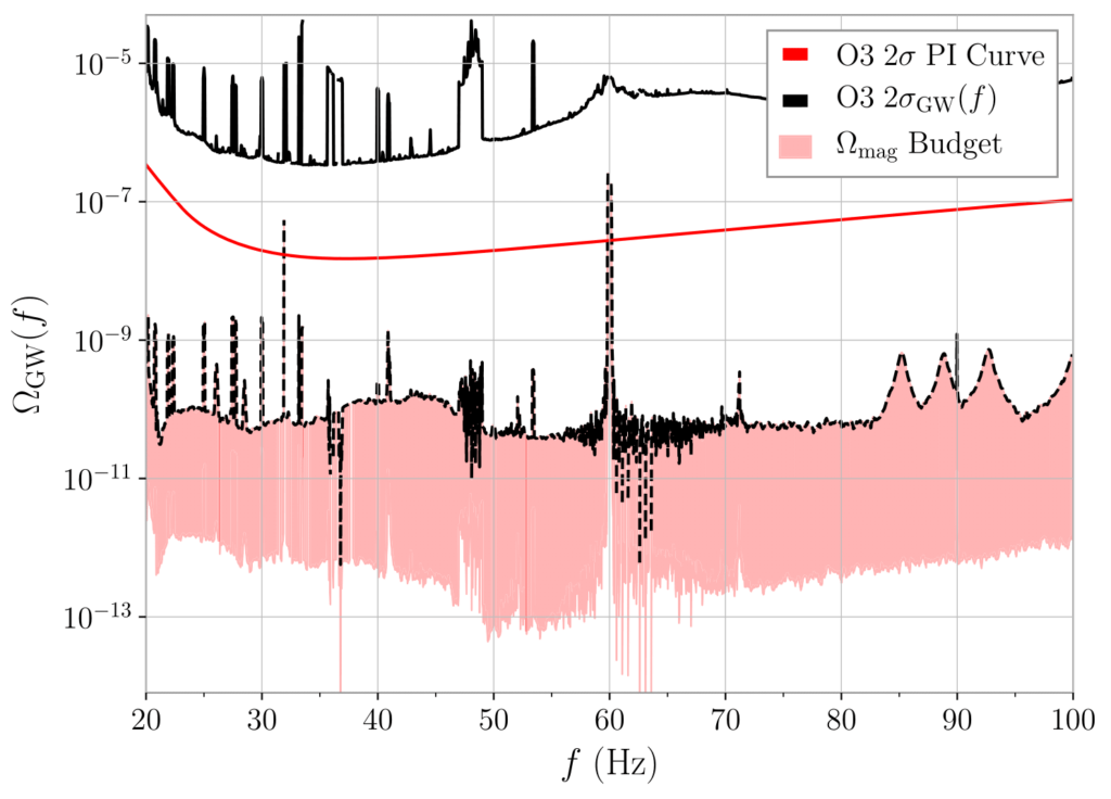
Figure 2: This plot shows the effect of the correlated magnetic signal, called ΩMag Budget (expressed in terms of the energy density of gravitational waves that would be inferred from this correlated signal in the interferometers, ΩGW), both for individual frequency bins (black dashed curve) as well as the integrated effect over multiple frequency bins (red band). The top of the red band (the black dashed curve) is below the black sensitivity curve, called 2σGW(f), indicating that magnetic contamination is well below our sensitivity in each individual frequency bin. The red sensitivity curve, called 2σ PI Curve, shows the sensitivity of the search to an accumulation of magnetic noise over multiple frequency bins. We see the red band is well below this red sensitivity curve. Our measured estimates of correlated magnetic noise are well below the sensitivity we achieve in O3, both in individual frequencies and when accounting for a sum over multiple frequencies.
We also determined upper limits on a scalar or vector polarized GW background. These are “forbidden” polarizations in general relativity (GR) where only tensor polarized GWs are allowed. Observing alternative polarizations would indicate that Einstein’s theory of general relativity should be modified to something more complicated. These searches for beyond-GR polarizations have benefited from the addition of Virgo data, since adding more detectors to the network can help distinguish between different polarizations. We have not found evidence of these “forbidden” polarizations. Other GW observations are also consistent with GWs having purely tensor polarizations, notably the observation of the binary neutron star signal GW170817.
We also use a model to predict the GWB due to compact binaries (see Figure 3), which may be the first source of the GWB that LIGO and Virgo can detect, as discussed here. We incorporated the most recent observations from the LIGO-Virgo catalog GWTC-2. We found that the GWB can potentially be detected by an upgraded version of the current detectors known as LIGO A+ and Advanced Virgo Plus. We also applied a joint analysis to the GWB and observations of individual compact binaries. Since the GWB is sensitive to binary mergers at larger distances than the individually detectable compact binaries, it is possible that measurements of the GWB could improve measurements of the merger rate of binary black holes in the early universe. While this is not the case in O3, we show that the GWB may be useful in future runs.
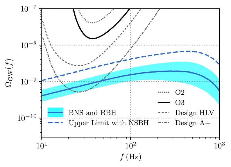
Figure 3: This plot compares the sensitivities of current and future observations with predictions for the background from unresolved CBCs, i.e., from binary neutron star (BNS) and binary black hole (BBH) mergers. The blue line is the median estimate of the strength of the GWB from BNS and BBH, while the light blue band is the 90% uncertainty region. Furthermore the sensitivities corresponding to the second and third observing runs (O2 and O3, respectively) are shown, as well as those corresponding to what we expect to achieve at design and A+ sensitivity (for the LIGO-Virgo network, HLV). The dashed blue line represents the 95% upper limit on the predicted CBC background obtained when including neutron star – black hole (NSBH) mergers. There are not yet any confirmed detections of NSBH mergers, so their rate of occurrence is more uncertain than that of BNSs or BBHs.
Despite the fact that we have been unable to claim a detection of a GWB -yet- this analysis was still a major step forward in our field. Many features were introduced for the first time in the analysis, such as the inclusion of data from a third interferometer, the use of gating to remove glitches, the integration of a fit for Schumann resonances in one consistent Bayesian framework and the use of a model to predict the GWB due to compact binaries. These new features might prove critical for future searches when we reach the sensitivity to claim a detection.
Find out more:
- Visit our websites:
- Read a free preprint of the full scientific article here.
- You will find more information on the general concept of gravitational waves here.
- Read more on the need to use multiple detectors.
- Find out what “forbidden” polarizations in general relativity are.
- Read more on compact binary coalescences (CBCs).